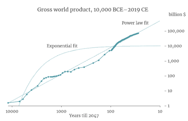
In arriving at our funding priorities—including criminal justice reform, farm animal welfare, pandemic preparedness, health-related science, and artificial intelligence safety—Open Philanthropy has pondered profound questions. How much should we care about people who will live far in the future? Or about chickens today? What events could extinguish civilization? Could artificial intelligence (AI) surpass human intelligence?
One strand of analysis that has caught our attention is about the pattern of growth of human society over many millennia, as measured by number of people or value of economic production. Perhaps the mathematical shape of the past tells us about the shape of the future. I dug into that subject. A draft of my technical paper is here. (Comments welcome.) In this post, I’ll explain in less technical language what I learned.
It’s extraordinary that the larger the human economy has become—the more people and the more goods and services they produce—the faster it has grown on average. Now, especially if you’re reading quickly, you might think you know what I mean. And you might be wrong, because I’m not referring to exponential growth. That happens when, for example, the number of people carrying a virus doubles every week. Then the growth rate (100% increase per week) holds fixed. The human economy has grown super-exponentially. The bigger it has gotten, the faster it has doubled, on average. The global economy churned out $74 trillion in goods and services in 2019, twice as much as in 2000.1 Such a quick doubling was unthinkable in the Middle Ages and ancient times. Surely early doublings took millennia.
If global economic growth keeps accelerating, the future will differ from the present to a mind-boggling degree. The question is whether there might be some plausibility in such a prospect. That is what motivated my exploration of the mathematical patterns in the human past and how they could carry forward. Having now labored long on the task, I doubt I’ve gained much perspicacity. I did come to appreciate that any system whose rate of growth rises with its size is inherently unstable. The human future might be one of explosion, an economic upwelling that eclipses the industrial revolution as thoroughly as it eclipsed the agricultural revolution. Or the future could be one of implosion, in which environmental thresholds are crossed or the creative process that drives growth runs amok, as in an AI dystopia. More likely, these impulses will mix.
I now understand more fully a view that shapes the work of Open Philanthropy. The range of possible futures is wide. So it is our task as citizens and funders, at this moment of potential leverage, to lower the odds of bad paths and raise the odds of good ones.
1. The human past, coarsely quantified
Humans are better than viruses at multiplying. If a coronavirus particle sustains an advantageous mutation (lowering the virulence of the virus, one hopes), it cannot transmit that innovation to particles around the world. But humans have language, which is the medium of culture. When someone hits upon a new idea in science or political philosophy (lowering the virulence of humans, one hopes) that intellectual mutation can disseminate quickly. And some new ideas, such as the printing press and the World Wide Web, let other ideas spread even faster. Through most of human history, new insights about how to grow wheat or raise sheep ultimately translated into population increases. The material standard of living did not improve much and may even have declined. In the last century or so, the pattern has flipped. In most of the world, women are having fewer children while material standards are higher for many, enough that human economic activity, in aggregate, has continued to swell. When the global economy is larger, it has more capacity to innovate, and potentially to double even faster.
To the extent that superexponential growth is a good model for history, it comes with a strange corollary when projected forward: the human system will go infinite in finite time. Cyberneticist Heinz Von Foerster and colleagues highlighted this implication in 1960. They graphed world population since the birth of Jesus, fit a line to the data, projected it, and foretold an Armageddon of infinite population in 2026. They evidently did so tongue in cheek, for they dated the end times to Friday the 13th of November. As we close in on 2026, the impossible prophecy is not looking more possible. In fact, the world population growth rate peaked at 2.1%/year in 1968 and has since fallen by half.
That a grand projection went off track so fast should instill humility in anyone trying to predict the human trajectory. And it’s fine to laugh at the absurdity of an infinite doomsday. Nevertheless, those responses seem incomplete. What should we make of the fact that good models of the past project an impossible future? While population growth has slowed, growth in aggregate economic activity has not slackened as much. Historically poor countries such as China are catching up with wealthier ones, adding to the global totals. Of course, there is only so much catching up to do. And economically important ideas may be getting harder to find. For instance, keeping up with Moore’s law of computer chip improvement is getting more expensive. But history records other slowdowns, each of which ended with a burst of innovation such as the European Enlightenment. Is this time different? It’s possible, to be sure. But it’s impossible to be sure.
Since 1960, when Von Foerster and colleagues published, other analysts have worked the same vein—now including me. I was influenced by writings of Michael Kremer in 1993 and Robin Hanson in 2000. Building on work by demographer Ronald Lee, Kremer brought ideas about “endogenous technology” (explained below) to population data like that of Von Foerster and his coauthors. Except Kremer’s population numbers went back not 2,000 years, but a million years. Hanson was the first to look at economic output, rather than population, over such a stretch, relying mainly on numbers from Brad De Long.
You might wonder how anyone knows how many people lived in 5000 BCE and how much “gross product” they produced. Scholars have formed rough ideas from the available evidence. Ancient China and Rome conducted censuses, for example. McEvedy and Jones, whose historical population figures are widely used, put it this way:
[T]here is something more to statements about the size of classical and early medieval populations than simple speculation….[W]e wouldn’t attempt to disguise the hypothetical nature of our treatment of the earlier periods. But we haven’t just pulled numbers out of the sky. Well, not often.
Meanwhile, until 1800 most people lived barely above subsistence; before then the story of GWP growth was mostly the story of population growth, which simplifies the task of estimating GWP through most of history.
I focused on GWP from 10,000 BCE to 2019. I chose GWP over population because I think economic product is a better indicator of capacity for innovation, which seems central to economic history. And I prefer to start in 10,000 BCE rather 1 million or 2 million years ago because the numbers become especially conjectural that far back. In addition, it seems problematic to start before the evolution of language 40,000–50,000 years ago. Arguably, it was then that the development of human society took on its modern character. Before, hominins had developed technologies such as handaxes, intellectual mutations that may have spread no faster than the descendants of those who wrought them. After, innovations could diffuse through human language, a novel medium of arbitrary expressiveness—one built on a verbal “alphabet” whose letters could be strung together in limitless, meaningful ways. Human language is the first new, arbitrarily expressive medium on Earth since DNA.2
Here is the data series I studied the most3:
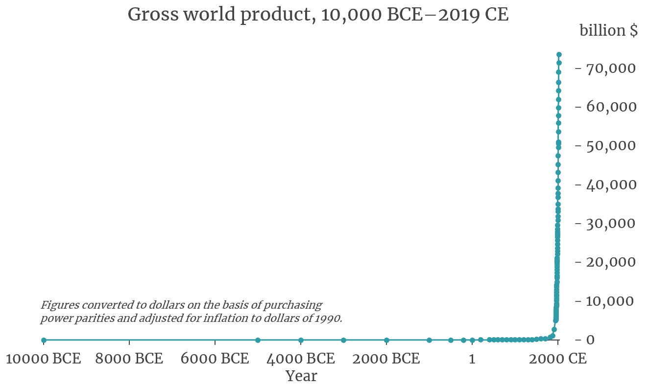
The series looks like a hockey stick. It starts at $1.6 billion in 10,000 BCE, in inflation-adjusted dollars of 1990: that is 4 million people times $400 per person per year, Angus Maddison’s quantification of subsistence living.
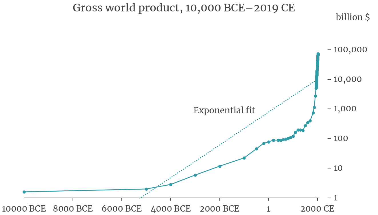
For clarity, here is the same graph but with $1 billion, $10 billion, $100 billion, etc., equally spaced. When the vertical axis is scaled this way, exponentially growing quantities—ones with fixed doubling times—follow straight lines. So to show how poorly human history corresponds to exponential growth, I’ve also drawn a best-fit line:
Finally, just as in that 1960 paper, I do something similar to the horizontal axis, so that 10,000, 1,000, 100, and 10 years before 2047 are equally spaced. (Below, I’ll explain how I chose 2047.) The horizontal stretching and compression changes the contour of the data once again. And it bends the line that represented exponential growth. But I’ve fit another line under the new scaling:
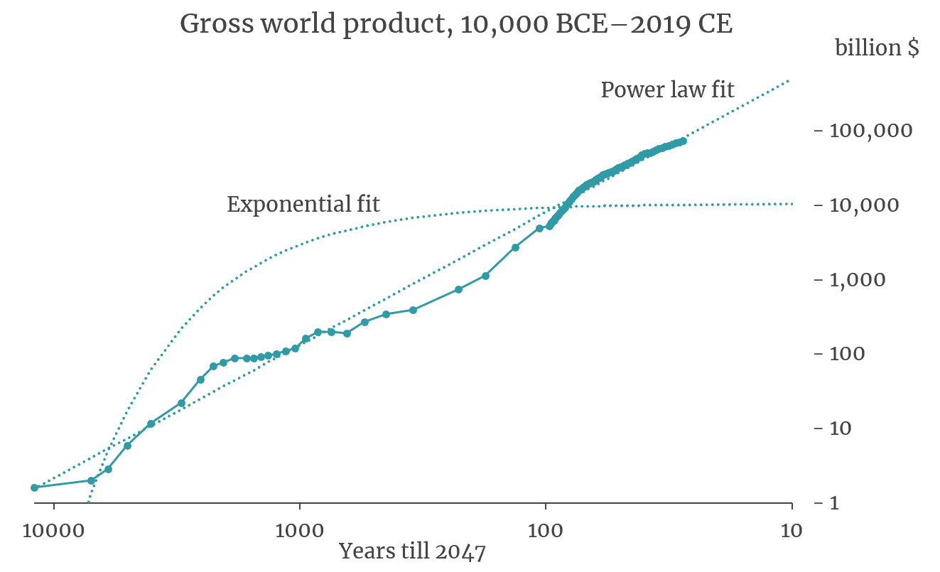
The new “power law” line follows the data points remarkably well. The most profound developments since language—the agricultural and industrial revolutions—shrink to gentle ripples on a long-term climb.
This graph raises two important questions. First, did those economic revolutions constitute major breaks with the past, which is how we usually think of them, or were they mere statistical noise within the longer-term pattern? And where does that straight line take us if we follow it forward?
I’ll tackle the second question first. I’ve already extended the line on the graph to 10 years before 2047, i.e., 2037, at which time it has GWP reaching a stupendous $500 trillion. That is ten times the level of 2007. If like Harold with his purple crayon you extend the line across your computer screen, off the edge, and into the ether, you will come to 1 year before 2047, then 0.1 before, then 0.01…. Meanwhile GWP will grow horrifically: to $30.7 quadrillion at the start of 2046, to $1.9 quintillion 11 months later, and so on. Striving to reach 2047, you will drive GWP to infinity.4 That was Von Foerster’s point back in 1960: explosion is an inevitable implication of the straight-line model of history in that last graph.
Yet the line fits so well. To grapple with this paradox, I took two main analytical approaches. I gained insight from each. But in the end the paradox essentially remained, and I think now that it is best interpreted in a non-mathematical way. I will discuss these ideas in turn.
2. Capturing the randomness of history
An old BBC documentary called the Midas Formula (transcript) tells how three economists in the early 1970s developed the E = mc2 of finance. It is a way to estimate the value of options such as the right to buy a stock at a set price by a set date. Fischer Black and Myron Scholes first arrived, tentatively, at the formula, then consulted Robert Merton. Watch till 27:40, then keep reading this post!
The BBC documented the work of Black, Scholes, and Merton not only because they discovered an important formula, but also because they co-founded the hedge fund Long-Term Capital Management to apply some of their ideas, and the fund imploded spectacularly in 1998.
In thinking about the evolution of GWP over thousands of years, I experienced something like what Merton experienced, except for the bits about winning a Nobel and almost bringing down the global financial system. I realized I needed a certain kind of math, then discovered that it exists.
The calculus of Isaac Newton and Gottfried Leibniz excels at describing smooth arcs, such as the path of Halley’s Comet. Like the rocket in the BBC documentary, the comet’s mathematical situation is always changing. As it boomerangs across the solar system, it experiences a smoothly varying pull from the sun, strongest at the perihelion, weakest when the comet sails beyond Neptune. If at some moment the comet is hurtling by the sun at 50 kilometers per second, then a second later, or a nanosecond later, it won’t be, not exactly. And the rate at which the comet’s speed is changing is itself always changing.
One way to approximate the comet’s path is to program a computer. We could feed in a starting position and velocity, code formulas for where the object will be a nanosecond later given its velocity now, update its velocity at the new location to account for the sun’s pull, and repeat. This method is widely used. The miracle in calculus lies in passing to the limit, treating paths through time and space as accumulations of infinitely many, infinitely small steps, which no computer could simulate because no computer is infinitely fast. Yet passing to the infinite limit often simplifies the math. For example, plotting the smooth lines and curves in the graphs above required no heavy-duty number crunching even though the contours represent growth processes in which the absolute increment, additional dollars of GWP, is always changing.
But classical calculus ignores randomness. It is great for modeling the fall of apples; not so much for the price of Apple. And not so much for rockets buffeted by turbulence, nor for the human trajectory, which has sustained shocks such as the fall of Rome, the Black Death, industrial take-off, world wars, depressions, and financial crises. It was Kyosi Itô who in the mid-20th century, more than anyone else, found a way to infuse randomness into calculus. The result is called the stochastic calculus, or the Itô calculus. (Though to listen to the BBC narrator, you’d think he invented the classical calculus rather than adding randomness to it.)
Think of an apple falling toward the surface of a planet whose gravity is randomly fluctuating, jiggling the apple’s acceleration as it descends. Or think of a trillion molecules of dry ice vapor released to careen and scatter across a stage. Each drop of an apple or release of a molecule would initiate a unique course through space and time. We cannot predict the exact paths but we can estimate the distribution of possibilities. The apple, for example, might more likely land in the first second than in the 100th.
I devised a stochastic model for the evolution of GWP. I borrowed ideas from John Cox, who as a young Ph.D. followed in the footsteps of Black, Scholes, and Merton. The stochastic approach intrigued me because it can express the randomness of human history, including the way that unexpected events send ripples into the future. Also, for technical reasons, stochastic models are better for data series with unevenly spaced data points. (In my GWP data, the first two numbers are 5,000 years apart, for 10,000 and 5,000 BCE, while the last two are nine apart, for 2010 and 2019.) Finally, I hoped that a stochastic model would soften the paradox of infinity: perhaps after fitting to the data, it would imply that infinite GWP in finite time was possible but not inevitable.
The equation for this stochastic model generalizes that implied by the straight “power law” line in the third graph above, the one we followed toward infinity in 2047.5 It preserves the possibility that growth can rise more than proportionally with the level of GWP, so that doublings will tend to come faster and faster. Here, I’ll skip the equations and stick to graphs.
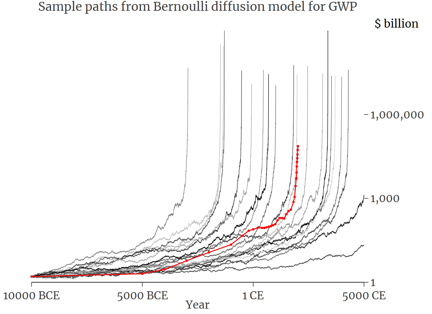
The first graph shows twenty “rollouts” of the model after it has been calibrated to match GWP history.6 All twenty paths start where the real data series starts, at $1.6 billion in 10,000 BCE. The real GWP series is in red. Arguably the rollouts meet the Goldilocks test: they resemble the original data series, but not so perfectly as to look contrived. Each represents an alternative history of humanity. Like the real series, the rollouts experience random ups and downs, woven into an overall tendency to rise at a gathering pace. I think of the downs as statistical Black Deaths. The randomness suffices to greatly affect the timing of economic takeoff: one rollout explodes by 3000 BCE while others do not do so even by 5000 CE. In a path that explodes early, I imagine, the wheel was invented a thousand years sooner, and the breakthroughs snowballed from there.
The second graph introduces a few changes. Instead of 20 rollouts, I run 10,000. Since that is too many to plot and perceive, I show percentiles. The black curve in the middle shows the median simulated GWP at each moment—the 50th percentile. Boundaries between grey bands mark the 5th, 10th, 15th, etc., percentiles. I also run 10,000 rollouts from the endpoint of the data series, which is $73.6 trillion in 2019, and depict those in the same way. And to take account of the uncertainty in the fitting of my model to the data, each path is generated under a slightly different version of the model.7 So this graph contains two kinds of randomness: the randomness of history itself, and the imprecision in our measurement of it.8
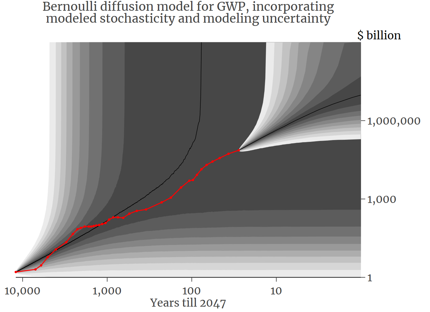
The actual GWP series, still in red, meanders mainly between the 40th and 60th percentiles. This good fit is the stochastic analog to the good fit of the power law line in the third graph in the earlier triplet. As a result, this model is the best statistical representation I have seen of world economic history, as proxied by GWP. That and a dollar will buy you an apple.
Through the Itô calculus, I quantified the probability and timing of escalation to infinity (according to the fitted model). The probability that a path like those in the first of the two graphs just above will not eventually explode is a mere 1 in 100 million. The median year of explosion is 1527. Applying the same calculations starting from 2019—that is, incorporating the knowledge that GWP reached $73.6 trillion last year—the probability of no eventual explosion falls to 1 in 1069, which is an atoms-in-the-universe sort of figure. (OK, there may be 1086 atoms. But who’s counting?) The estimate of the median explosion year sharpens to 2047 (95% confidence range is ±16 years), which is why I used 2047 in the third graph of the post. In the mathematical world of the best-fit model, explosion is all but inevitable by the end of the century.9
Incorporating randomness into the modeling does not after all soften the paradox of infinity. An even better mathematical description of the past still predicts an impossible future.
I will put that conundrum back on hold for the moment and address the other question inspired by the power law’s excellent fit to the GWP numbers. Should the agricultural and industrial revolutions be viewed as ruptures in history or as routine, modest deviations around a longer-term trend? To assess whether GWP was surprisingly high in 1820, by which time the industrial revolution had built a head of steam, I fitted the model just to the data before 1820, i.e., through 1700. Then I generated many paths wiggling forward from 1700 to 1820. The 1820 GWP value of $741 billion places it in the 95th percentile of these simulated paths: the model is “surprised,” going by previous history, at how big GWP was in 1820. I repeat the whole exercise for other time points, back to 1600 and forward to 2019. This graph contains the results:
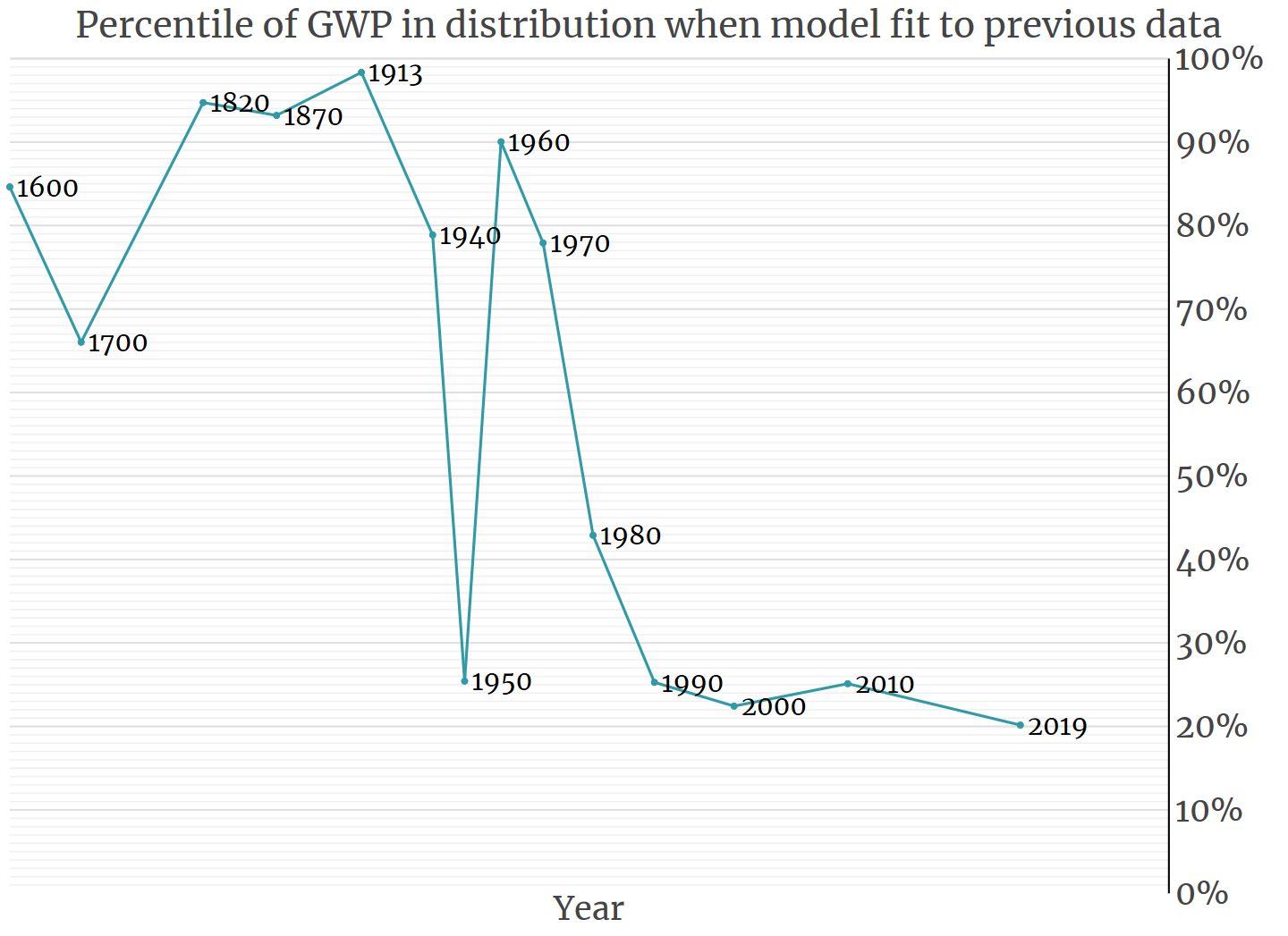
The model is also surprised by the data point after 1820, for 1870, despite “knowing” about the fast GWP growth leading up to 1820. And it is surprised again in 1913. Now, if my stochastic model for GWP is correct, then the 14 dots in this graph should be distributed roughly evenly across the vertical 0–100% range, with no correlation from one dot to the next. That’s not what we see. The three dots in a row above the 90th percentile strongly suggests that the economic growth of the 19th century broke with the past. The same goes for the four low values since 1990: recent global growth has been slower and steadier than the model predicts from previous history.
In sum, my stochastic model succeeds in expressing some of the randomness of history, along with the long-term propensity for growth to accelerate. But it is not accurate or flexible enough to fully accommodate events as large and sudden as the industrial revolution. Nevertheless, I think it is a virtue, and perhaps an inspiration for further work, that this rigorous model can quantify its own shortcomings.
3. Land, labor, capital, and more
To this point I have represented economic growth as univariate. A single quantity, GWP, determines the rate of its own growth, if with randomness folded in. I have radically caricatured human history—the billions of people who have lived, and how they have made their livings. That is how models work, simplifying matters in order to foreground aspects few enough for the mind to embrace.
A longstanding tradition in the study of economic growth is to move one notch in the direction of complexity, from one variable to several. Economic activity is cast as combining “factors of production.” Thus we have inherited from classical economists such as Adam Smith and David Ricardo the triad of land, labor, and capital. Modern factor lists may include other ingredients, such as “human capital,” which is investment in skills and education that raises the value of one’s labor. A stimulus to one factor can boost economic output, which can be reinvested in some or all of the factors: more office buildings, more college degrees, more kids even. In this way, factors can propel their own growth and each other’s, in a richer version of the univariate feedback loop contemplated above. And just as in the univariate model that fits GWP history so well, the percentage growth rate of the economy can increase with output.10
I studied multivariate models too11 though I left for another day the technically daunting step of injecting them with randomness. I learned a few things.
First, the single-variable “power law” model—that straight line in my third graph up top—is, mathematically, a special case of standard models in economics, models that won at least one Nobel (for Robert Solow) and are taught to students every day somewhere on this Earth.12 In this sense, fitting the power law model to the GWP data and projecting forward is not as naive as it might appear.
To appreciate the concern about naiveté, think of the IHME model of the spread of coronavirus in the United States. It received much attention—including criticism that it is an atheoretical “curve-fitting” exercise. The IHME model worked by synthesizing a hump-shaped contour from the experiences of Wuhan and Italy, then fitting the early section of the contour to U.S. data and projecting forward. The IHME exercise did not try to mathematically reconstruct what underlay the U.S. data, the speed at which the virus hopped from person to person, community to community. If “the IHME projections are based not on transmission dynamics but on a statistical model with no epidemiologic basis,” the analogous charge cannot so easily be brought against the power law model for GWP. It is in a certain way rooted in established economics.
The second thing I learned constitutes a caveat that I just glossed over. By the mid-20th century, it became clear to economists that reinvestment alone had not generated the economic growth of the industrial era. Yes, there were more workers and factories, but from any given amount of labor and capital, industrial countries extracted more value in 1950 than in 1870. As Paul Romer put it in 1990,
The raw materials that we use have not changed, but…the instructions that we follow for combining raw materials have become vastly more sophisticated. One hundred years ago, all we could do to get visual stimulation from iron oxide was to use it as a pigment. Now we put it on plastic tape and use it to make videocassette recordings.
So in the 1950s economists inserted another input into their models: technology. As meant here, technology is knowledge rather than the physical manifestations thereof, the know-how to make a smartphone, not the phone itself.
The ethereal character of technology makes it alchemical too. One person’s use of a drill bit or farm plot tends to exclude others’ use of the same, while one person’s use of an idea does not. So a single discovery can raise the productivity of the entire global economy. I love Thomas Jefferson’s explanation, which I got from Charles Jones:
Its peculiar character … is that no one possesses the less, because every other possesses the whole of it. He who receives an idea from me, receives instruction himself without lessening mine; as he who lights his taper at mine, receives light without darkening me. That ideas should freely spread from one to another over the globe, for the moral and mutual instruction of man, and improvement of his condition, seems to have been peculiarly and benevolently designed by nature, when she made them, like fire, expansible over all space, without lessening their density at any point.
That ideas can spread like flames from candle to candle seems to lie at the heart of the long-term speed-up of growth.
And the tendency to speed up, expressed in a short equation, is also what generates the strange, superexponential implication that economic output could spiral to infinity in decades. Yet that implication is not conventional within economics, unsurprisingly. Since the 1950s, macroeconomic modeling has emphasized the achievement of “steady state,” meaning a constant economic growth rate such as 3% per year. Granted, even such exponential growth seems implausible if we look far enough ahead, just as the coronavirus case count can’t keep doubling forever. But, in their favor, models predicting steady growth cohered with the relatively stability of per-person economic growth over the previous century in industrial countries (contrasting with the acceleration we see over longer stretches). And under exponential growth the economy merely keeps expanding; it does not reach infinity in finite time. “It is one thing to say that a quantity will eventually exceed any bound,” Solow once quipped. “It is quite another to say that it will exceed any stated bound before Christmas.”
The power law model that fits history so well, yet explodes before Christmas, is mathematical kin with Solow’s influential models. So how did he avoid the explosive tendencies? To understand, step over to my whiteboard, where I’ll diagram a typical version of Solow’s model. The economy is conceived as a giant factory with four inputs: labor, capital, human capital, and technology. It produces output, much of which is immediately eaten, drunk, watched, or otherwise consumed:
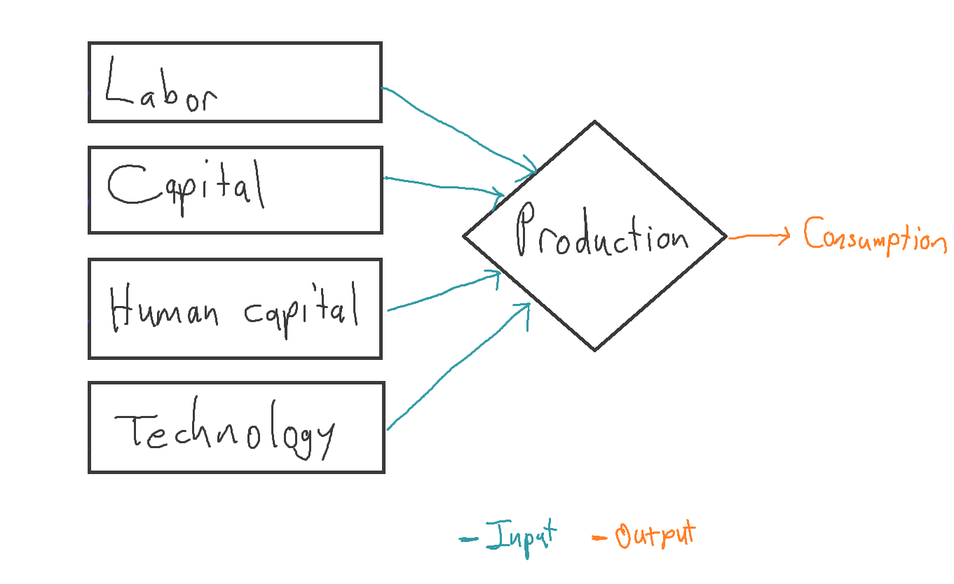
Some of the output is not consumed, and is instead invested in factors—here, the capital of businesses, and the human capital that is skills in our brains:
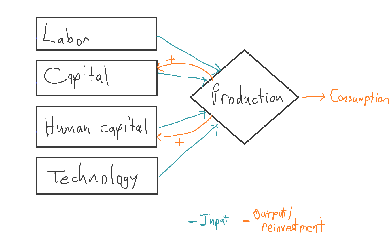
A final dynamic is depreciation: factories wear out, skills fade. And the more there are, the more wear out each year. So just below I’ve drawn little purple loops to the left of these factors with minus signs inside them. Fortunately, the reinvestment flowing in through the orange arrows can compensate for depreciation by effecting repairs and refreshing skills.
Now, labor and technology can also depreciate, since workers age and die and innovations are occasionally lost too. But Solow put the sources of their replenishment outside his model. From the standpoint of the Solow model, they grow for opaque reasons. So they receive no orange arrows. And to convey their unexplained tendency to grow, I’ve drawn plus signs in their purple feedback loops:
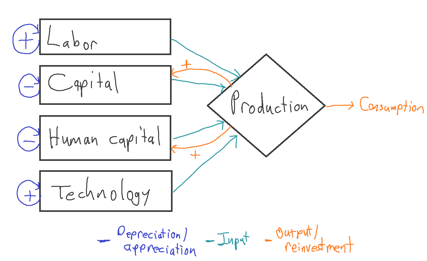
In the language of economics, Solow made technology and labor exogenous. This choice constitutes another caveat to my claim that the power law model is rooted in standard economic models. If the factors growing at a fixed, exogenously determined rate are economically important enough, they can keep the whole system from exploding into infinite growth.
For Solow, the invocation of exogeneity had two virtues and a drawback. I’ll explain them with reference to technology, the more fateful factor.
One virtue was humility: it left for future research the mystery of what sets the pace of technological advance.13
The other virtue was that defaulting to the simple assumption that technology—the efficiency of turning inputs into output—improved at a constant rate such as 1% per year led to the comfortable prediction that a market economy would converge to a “steady state” of constant growth. It was as if economic output were a ship and technology its anchor; and as if the anchor were not heavy enough to moor the ship, but its abrasion against the seabed capped the ship’s speed. In effect, Solow built the desired outcome of constant growth into his model.
In general, the drawback of casting technology as exogenous is that it leaves a story of long-term economic development incomplete. It does not explain or examine where technical advance comes from, nor its mathematical character, despite its centrality to history. On its face, taking the rate of technological advance as fixed implies, implausibly, that a society’s wealth has zero effect on its rate of technical advance. There is no orange arrow from Production to Technology. Yet in general, when societies become richer, they do invest more in research and development and other kinds of innovation. It was this observation that motivated Romer, among others, to reconfigure economic models to make technological advance endogenous (which eventually earned a Nobel too). Just as people can invest earnings into capital, people can invest in technology, not to mention labor (in the number, longevity, and health of workers). In the set-up on my whiteboard, making these links merely requires writing the same equations for technology and labor as for capital. It is like drawing the sixth branch of a snowflake just like the other five. It looks like this:
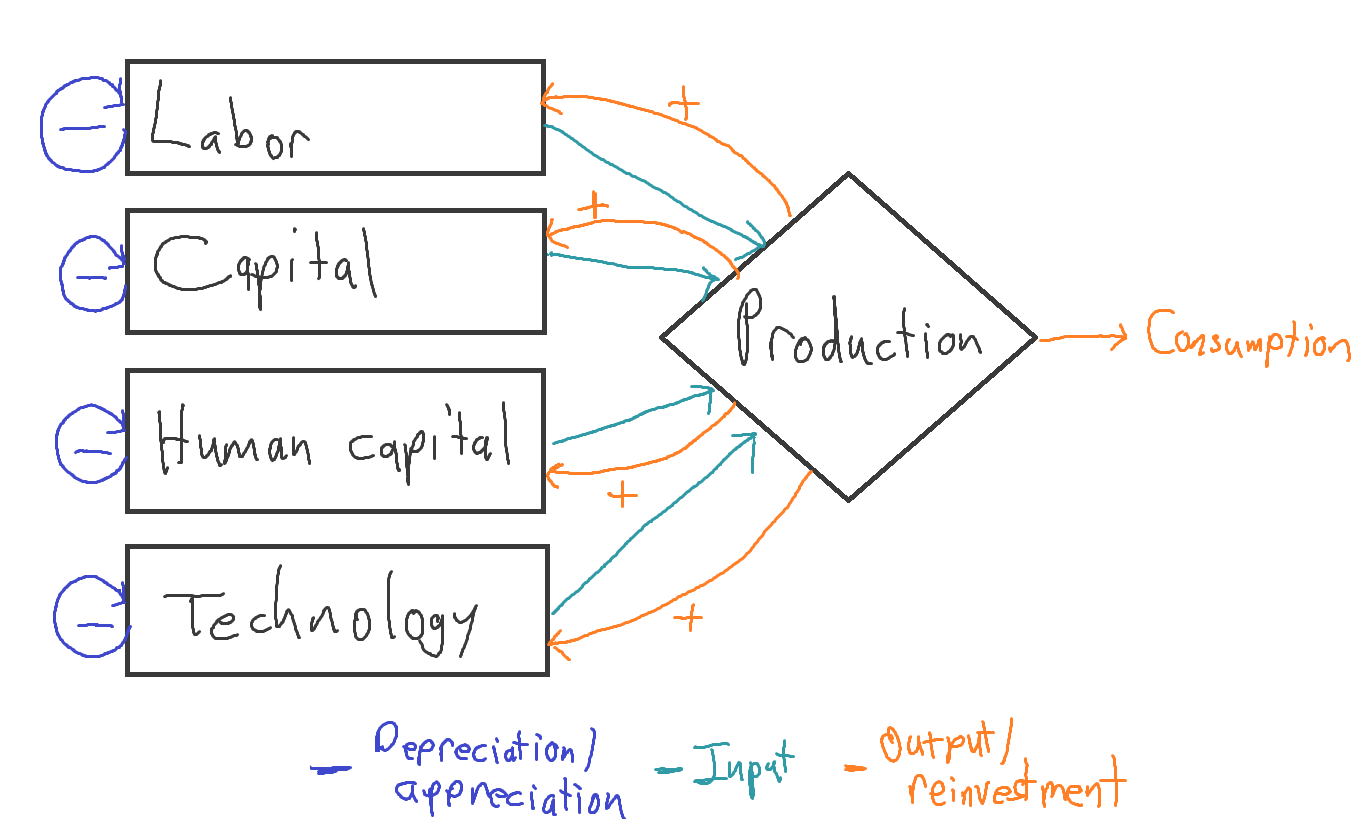
I discovered that when you do this—when you allow technology and all the other factors to affect economic output and be affected by it—the modeled system is unstable. (I was hardly the first to figure that out.) As time passes, the amount of each factor either explodes to infinity in finite time or decays to zero in infinite time. And under broadly plausible (albeit rigid) assumptions about the rates at which that Production diamond transforms inputs into output and reinvestment, explosion is the norm. It can even happen when ideas are getting harder to find. For example, even though it is getting expensive to squeeze more speed out of silicon chips, the global capacity to invest in the pursuit has never been greater.14
Here’s a demonstration of how endogenous technology creates explosive potential. Imagine an economy that begins with 1 unit each of labor, capital, human capital, and technology. Define the “units” how you please. A unit of capital could be a handaxe or a million factories. Suppose the economy then produces 1 unit of output per year. I’ve diagrammed that starting point by writing a 1 next to each factor as well as to the right of the Production diamond. To simplify, I’ve removed the purple depreciation loops:
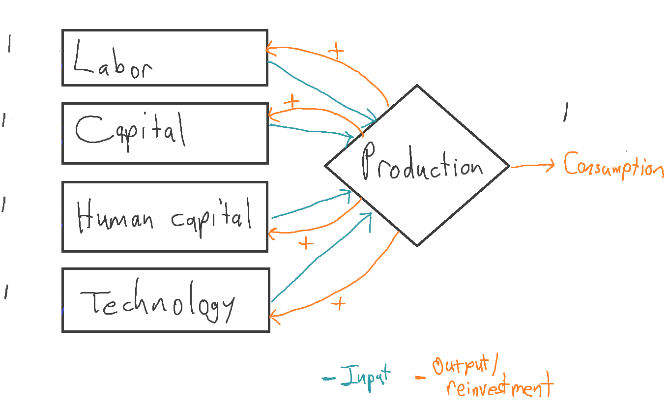
Now suppose that over a generation, enough output is reinvested in each factor other than technology that the stock of each increases to 2 units. Technology doesn’t change. Doubling the number of factories, workers, and diplomas they collectively hold is like duplicating the global economy: with all the inputs doubled, output should double too:
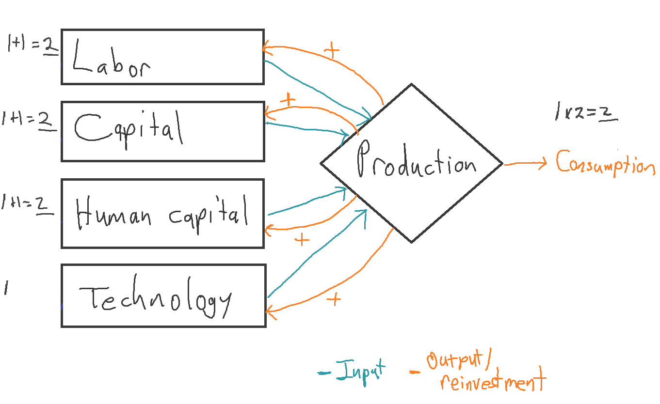
Now suppose that in addition over this same generation, the world invests enough in R&D to double technology. Now the world economy extracts twice the economic value from given inputs—which themselves have doubled. So output quadruples in the first generation:
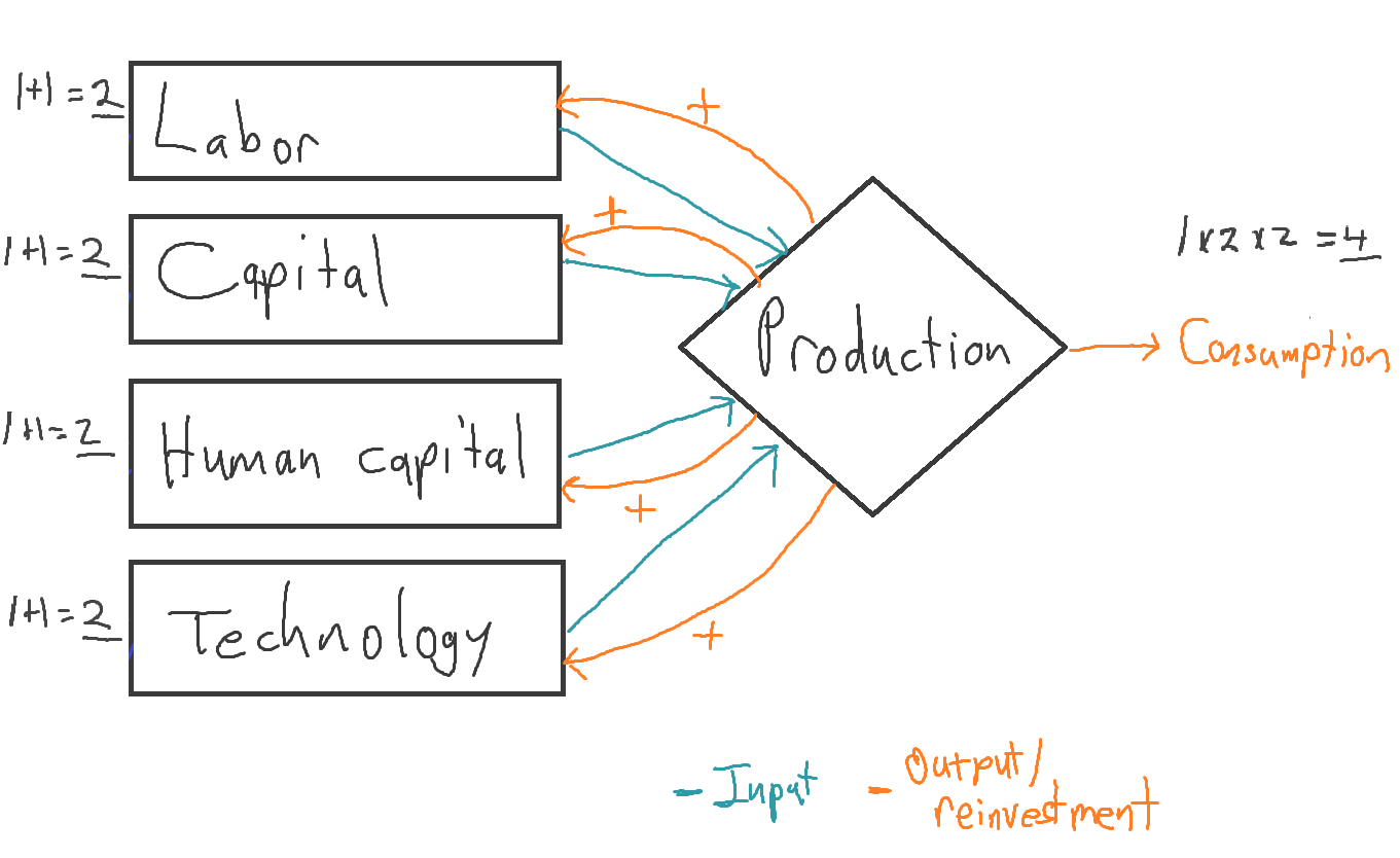
What happens when the process repeats? Since output starts at 4 per year, instead of 1 as in the previous generation, total reinvestment into each input also quadruples. So where each factor stock climbed by 1 unit in the first generation, now each climbs by 4, from 2 to 6. In other words, each input triples by the end of this generation. And just as doubling each input, including technology, multiplied output by 2×2 = 4, the new cycle multiplies output by 3×3 = 9, raising it from 4 to 36:
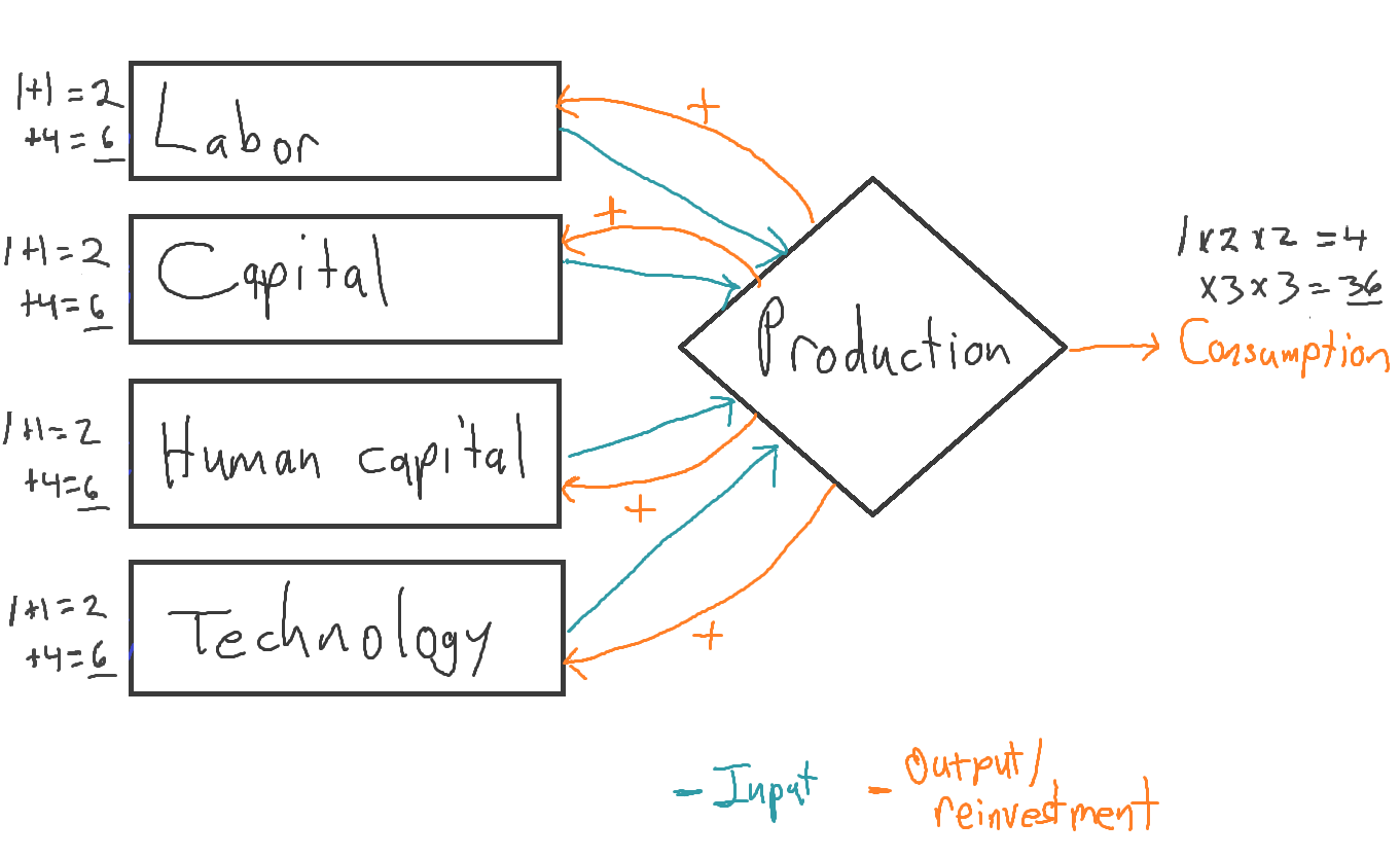
The growth rate accelerates. The doubling time drops. And it drops ever more in succeeding generations.
Again, it is technology that drives this acceleration. If technology were stagnant, or if, as in Solow’s model, its growth rate were locked down, the system could not spiral upward so.
In the paper, I carry out a more intense version of this exercise, with 100 million steps, each representing 10 minutes. I imagine the economy to start in the Stone Age, so I endow it with a lot of labor (people) but primitive technology and little capital or human capital. I start population at 1 (which could represent 1 million) and the other factors lower. This graph shows how factor stocks and economic output (GWP) evolve over time:
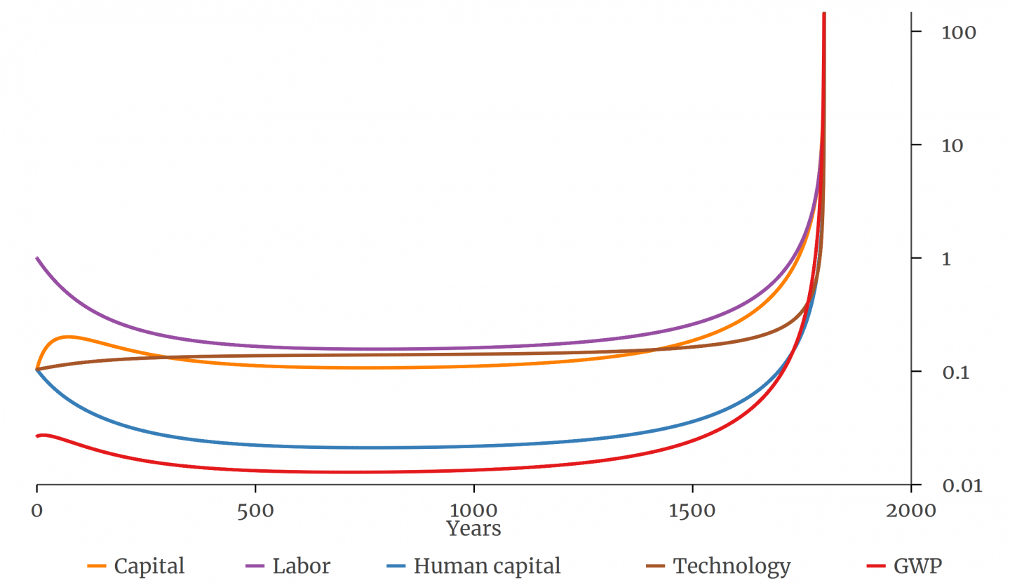
Apparently my simulated economy could not support all the people I gave it at the start, at least given the fraction of its income I allowed it to invest in creating and sustaining life. So population falls at first, until after about 500 years the economy settles into something close to stasis. But it is not quite stasis, for eventually the economy starts to grow perceptibly, and within a few centuries its scale ascends to infinity. The sharp acceleration resembles history.
It turns out that a superexponential growth process not only fits the past well. It is rooted in conventional economic theory, once that theory is naturally generalized to allow for investment in technology.
4. Interpreting infinity
How then are we to make sense of the fact that good models of the past predict an impossible future?
One explanation is simply that history need not repeat itself. The best model for the past may not be the best for the future. Perhaps technology can only progress so far. It has been half a century since men first stepped onto the moon and the 747 entered commercial service; contrast that with the previous half century of progress in aeronautics. As we saw, the world economy has grown more slowly and steadily in the last 50 years than the univariate model predicts. But it is hard to know whether any slowdown is permanent or merely a century-scale pause.
A deeper take is that infinities are a sign not that a model is flatly wrong but that it loses accuracy outside a certain realm of possible states of the world. Beyond that realm, some factor once neglected no longer can be. Einstein used the fact that the speed of light is the same in all inertial reference frames to crack open classical physics. It turned out that when such great speeds were involved, the old equations become wrong. As Anders Johansen and Didier Sornette have written,
Singularities are always mathematical idealisations of natural phenomena: they are not present in reality but foreshadow an important transition or change of regime. In the present context, they must be interpreted as a kind of ‘critical point’ signaling a fundamental and abrupt change of regime similar to what occurs in phase transitions.
What might be that factor once neglected that no longer can be? One candidate is a certain unrealism in calculus-based economic models. Calculus is great for predicting the path of comets, along which the sun’s pull really does change in each picosecond. All the the simulations I’ve graphed here treat innovation analogously, as something that happens in infinitely many steps, each of infinitely small size, each diffused around the globe at infinite speed. But real innovations take time to adopt, and time lags forestall infinities. If you keep hand-cranking the model on my white board, you won’t get to infinity by Christmas. You will just get really big numbers. That is because the simulation will take a finite number of chunky steps, not an infinite number of infinitely small steps.
The upshot of recognizing the unrealism of calculus, however, seems only to be that while GWP won’t go to infinity, it could still get stupendously big. How might that happen? We have in hand machines whose fundamental operations proceed a million times faster than those of the brain. And researchers are getting better at making such machines work like brains. Artificial intelligence might open major new production possibilities. More radically, if AI is doing the economic accounting a century from now, it may include the welfare of artificial minds in GWP. Their number would presumably dwarf the human population. As absurd as that may sound, a rise of AI could be seen as the next unfolding of possibilities that began with the evolution of talkative, toolmaking apes.
Another neglected factor is the flow of energy (more precisely, negative entropy) from the sun and the earth’s interior. As economists Nicholas Georgescu-Roegen and Herman Daly have emphasized, depictions of the economic process like my whiteboard diagrams obscure the role of energy and natural resources in converting capital and labor into output. For this reason, at the end of my paper, I add natural resources to the model, rather as the classical economists included land. Since sunlight is constantly replenishing the biosphere, I have natural resources appreciate rather than depreciate. And to capture how economic activity can deplete natural resources, I cast the “reinvestment” in resources as negative.15 This is conceptually awkward, but I don’t see a better way within this modeling structure. I indicate these dynamics with a positive sign in the purple loop for natural resources and a minus sign on its orange reinvestment arrow:
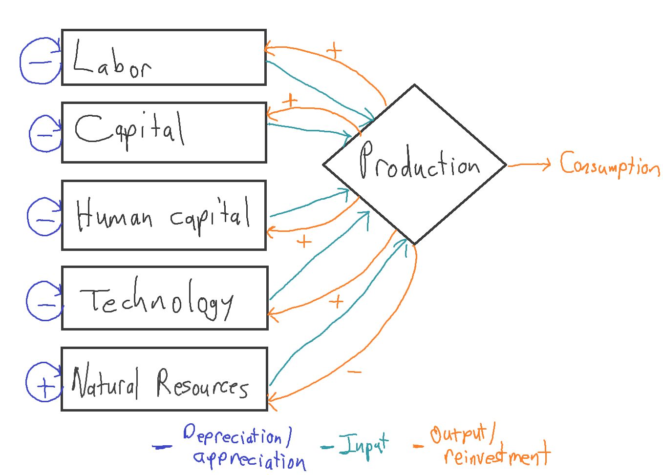
In the simulation, the stock of resources is taken as initially plentiful, so it too starts at 1 rather than a lower value. The slow, solar-powered increase in this economic input (in green) hastens the economic explosion by a thousand years. But because the growing economy depletes natural resources more rapidly, the take-off initiates a plunge in natural resources, which brings GWP down with it. In a flash, explosion turns into implosion.
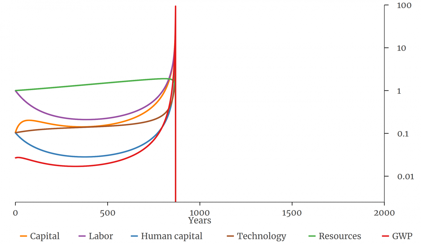
The scenario is, one hopes, unrealistic. Its realism will depend on whether the human enterprise ultimately undermines itself by depleting a natural endowment such as safe water supplies or the greenhouse gas absorptive capacity of the atmosphere; or whether we skirt such limits by, for example, switching to climate-safe energy sources and using them to clean the water and store the carbon.
…which points up another factor the model neglects: how people respond to changing circumstances by changing their behavior. While the model allows the amount of labor, capital, etc., to gyrate, it locks down the numbers that shape that evolution, such as the rate at which economic output translates into environmental harm. This is another reason to interpret the model’s behavior directionally, as suggesting a tendency to diverge, not as gesturing all the way to utopia or dystopia.
Still, this run suffices to demonstrate that an accelerating-growth model can capture the explosiveness of long-term GWP history without predicting a permanently spiraling ascent. Thus the presence of infinities in the model neglecting natural resource degradation does not justify dismissing superexponential models as a group. This too I learned through multivariate modeling.
5. Conclusion
I do not know whether most of the history of technological advance on Earth lies behind or ahead of us. I do know that it is far easier to imagine what has happened than what hasn’t. I think it would be a mistake to laugh off or dismiss the predictions of infinity emerging from good models of the past. Better to take them as stimulants to our imaginations. I believe the predictions of infinity tell us two key things. First, if the patterns of long-term history continue, some sort of economic explosion will take place again, the most plausible channel being AI. It wouldn’t reach infinity, but it could be big. Second, and more generally, I take the propensity for explosion as a sign of instability in the human trajectory. Gross world product, as a rough proxy for the scale of the human enterprise, might someday spike or plunge or follow a complicated path in between. The projections of explosion should be taken as indicators of the long-run tendency of the human system to diverge. They are hinting that realistic models of long-term development are unstable, and stable models of long-term development unrealistic. The credible range of future paths is indeed wide.
Data and code for the paper and for this post are on GitHub. The code runs in Stata. Open Philanthropy’s Tom Davidson wrote a Colab notebook that lets you perform and modify the stochastic model fitting in Python. A comment draft of the paper is here.
